Fine-Tuning a Model: Pros, Cons, and Where It Breaks
Teaching a Model to Read SystemVerilog presented the result: a GraphCodeBERT model fine-tuned on a 6,257-file SV/UVM corpus, achieving F1 = 0.972 overall. This article is about the cost of getting there and the walls you hit.
Fine-tuning is not a magic escalator from “general model that doesn’t understand SV” to “specialist model that does.” It’s a tradeoff surface with specific failure modes, and understanding those failure modes determines whether fine-tuning is the right move for your situation.
What fine-tuning actually did
Model: GraphCodeBERT-base (125M parameters, MIT license). Pre-trained on GitHub code across multiple languages; understands code structure better than general-purpose BERT but has no SV-specific training.
Task: Token classification. Label each token in a SV/UVM file as one of: MODULE, PORT, PARAMETER, COVERGROUP, PACKAGE, UVM_AGENT, UVM_DRIVER, UVM_MONITOR, UVM_SEQUENCER, UVM_ENV, UVM_SEQ, CLOCK_DOMAIN, or O (outside).
Corpus: 6,257 files, 1.27 million lines, 11 open-source repos (OpenTitan, Ibex, CVA6, AXI, common_cells, VeeR-EH1/EH2, uvm-core, core-v-verif, caliptra-rtl, cv32e40p, uvmBasics). All Apache 2.0 or MIT licensed.
Hardware: Apple M4 Pro 24GB, MPS backend. Training time approximately 18 minutes for 5 epochs.
Results at epoch 5:
| Entity | Precision | Recall | F1 |
|---|---|---|---|
| MODULE | 0.987 | 0.983 | 0.985 |
| PORT | 0.981 | 0.979 | 0.980 |
| PARAMETER | 0.972 | 0.968 | 0.970 |
| COVERGROUP | 1.000 | 1.000 | 1.000 |
| PACKAGE | 0.979 | 0.977 | 0.978 |
| UVM types (all) | n/a | n/a | ≈ 0.000 |
| Overall | 0.969 | 0.975 | 0.972 |
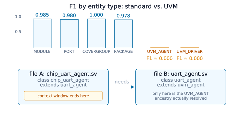
The gap between standard types (F1 ≈ 0.98) and UVM types (F1 ≈ 0.000) tells you exactly where fine-tuning helps and where it doesn’t.
Why the standard types work well
MODULE, PORT, PARAMETER, COVERGROUP, and PACKAGE are syntactically distinctive. A module declaration looks like a module declaration. A port list is a port list. These entities have clear lexical signatures that GraphCodeBERT can learn to recognize from surface patterns.
With 6,257 files and enough examples, the model learns these patterns reliably. Five epochs on M4 Pro took 18 minutes. The result is production-quality extraction for these types.
The mechanism here is essentially pattern recognition from training distribution. The model has seen thousands of module declarations and can identify the next one. This is fine-tuning at its best.
Why UVM types fail
UVM class identity is determined by inheritance, not syntax. Consider:
1class chip_uart_agent extends uart_agent;
2  // ...
3endclass
Is chip_uart_agent a UVM_AGENT? Only if uart_agent is. And uart_agent extends uvm_agent? Yes, but that declaration is in a different file. The token classifier sees chip_uart_agent in isolation; the uvm_agent ancestor is not in its local context window.
GraphCodeBERT processes token sequences within a context window. It can see local syntax. It cannot resolve multi-hop inheritance chains that span files. This is a structural limitation of the architecture, not a data quantity problem.
The test set had only 2 examples of UVM_AGENT (compared to 3,091 PORT examples). Partly that’s class imbalance; UVM component types are rarer than ports. But even with more data, a model that can’t see cross-file inheritance cannot learn to resolve it.
The class imbalance problem
Training data is not uniformly distributed:
| Entity | Training examples |
|---|---|
| PORT | ~40,000 |
| MODULE | ~15,000 |
| PARAMETER | ~8,000 |
| UVM_AGENT | < 50 |
| UVM_DRIVER | < 50 |
| CLOCK_DOMAIN | < 20 |
When your rarest entity type has fewer than 50 training examples, the model doesn’t see enough variance to generalize. It either learns to classify them (at the cost of false positives) or learns to ignore them (zero recall, which is what happened).
Weighted loss functions help at the margins. The fundamental problem is that UVM class declarations are sparse; they appear once per file, while port declarations appear dozens of times. More corpus data helps, but the ceiling on UVM type examples is set by how many UVM component classes exist in open-source SV repos, which is a small number.
The SV-specific preprocessing burden
Before training was even viable, significant preprocessing was required:
Generated file filtering. Register banks, RDL outputs, and auto-generated CSR files make up a substantial fraction of large SV repos. Including them inflates the PORT count (registers have many fields that look like ports) without adding useful training signal. The filter checks the first 1KB of each file for “do not edit” markers.
Comment handling. SV files contain large multi-line comment blocks: license headers, lengthy block comments, sometimes entire sections of commented-out code. Including them confuses the tokenizer. A blank_comments() pass is required before tokenization.
Verible integration. Getting parse trees out of Verible required combining --printtree and --export_json flags together. Using --export_json alone produces an error that isn’t clearly documented. This is the kind of thing that costs two hours before you find it in a GitHub issue thread.
None of this is intellectually hard, but it’s all load-bearing. Skipping any of it degrades training quality in ways that don’t always show up immediately.
What fine-tuning is actually buying you
The honest accounting:
What you get:
- Production-quality extraction for syntactically distinctive entities (F1 ≈ 0.98)
- A model that fits on a workstation (125M parameters, < 1GB VRAM)
- Fast inference: a few milliseconds per file, not seconds
- No API calls, full local deployment
- Embeddings that encode structural similarity (dma_ctrl / dma_engine = 0.94, dma_ctrl / axi_driver = 0.71)
What you don’t get:
- Reliable UVM type classification (F1 ≈ 0.000)
- Cross-file inheritance resolution
- Understanding of parameterized class instantiation
- Clock domain inference from structural analysis
- Anything that requires seeing across file boundaries
The entity types you don’t get are exactly the ones that make UVM testbenches navigable: agent types, driver/monitor/sequencer connections, sequence hierarchies. A model that finds every port but can’t identify the agents is a model that answers the wrong questions.
The architectural wall
GraphCodeBERT was designed for general code intelligence tasks, code search, clone detection, code summarization, across multiple languages. It works by encoding tokens and their data-flow graph within a context window.
For SV/UVM NER specifically, the bottleneck is cross-file reasoning. GraphCodeBERT doesn’t have a mechanism to resolve inheritance chains that span files. This isn’t something you can fix with more data or longer training; it’s a property of the architecture.
You can work around it with post-processing: extract all class A extends B declarations across the repo, build the inheritance graph separately, then propagate labels (if B is a uvm_agent, label A as UVM_AGENT). That produces correct labels in many cases. But it requires a separate resolution step, and it fails when parameterized types or conditional inheritance are involved.
The alternative is a model architecture that can see cross-file context, or one that was pre-trained specifically on SV with inheritance resolution baked into the pre-training task. That’s what Fine-Tuning Specialized Models for SV/UVM covers.
When fine-tuning is the right answer
Despite the UVM gap, fine-tuning GraphCodeBERT is the right move for certain use cases:
- Module inventory at scale. If you need to index all modules, parameters, and ports in a repo of thousands of files, this model does it accurately and locally in seconds.
- Embedding-based similarity search. The embeddings encode structural similarity correctly even when the NER labels are wrong.
dma_ctrlanddma_engineare close in embedding space because they have similar port signatures, regardless of their class hierarchy. - Base layer for a hybrid pipeline. Standard entities extracted by this model can be combined with a separate inheritance-resolution pass to produce the full UVM type classification.
Fine-tuning is not the end of the story. It’s the right tool for a subset of the problem, and knowing which subset keeps you from wasting time on the parts it can’t solve.